In this blog, I am going to use various R packages mainly from the tidyverse package by Hadley Wickham to analyze tweets from twitter archive of lordMwesh with a view of establishing his tweeting habits. The basis of the blog is a post by Julia Silge. lordMwesh is an ICT policy expert with vast experience in Internet governance.
Twitter archive is a nice large dataset with results that can be interesting and is good enough for those interested in learning R statistical language. To download your twitter data, browse to your Twitter Profile > Settings page, then click request your archive. A download link will be send to your email address that allows you download a .zip file which contains among other files, a nicely formated dataset of your tweets in form of an excel file.
The first step after obtaining the dataset was to load the tweets.csv file. A quick summary was able to show that lordMwesh had tweeted or retweeted 21,447 times since joining twitter.
How has lordMwesh’s been tweeting over the years?
We begin by formating the tweets timestamp using date functions from lubridate package. The ggplot package is then used to plot the tweet count over the years.
tweets$timestamp <- ymd_hms(tweets$timestamp)
tweets$timestamp <- with_tz(tweets$timestamp, "Africa/Nairobi")

ggplot(data = tweets, aes(x = year(timestamp))) +
  geom_histogram(breaks = seq(2008.5, 2018.5, by =1), aes(fill = ..count..)) +
  theme(legend.position = "none") +
  ggtitle("Tweeting pattern over the years")+
  xlab("Time") + ylab("Number of tweets") +
  scale_fill_gradient(low = "midnightblue", high = "aquamarine4")
lordMwesh joined twitter in 2009 with 2016 and 2012 being his most active years on twitter.
We then sought to identify his tweeting pattern by months, days of the week and time of the day.
ggplot(data = tweets, aes(x = month(timestamp, label = TRUE))) +
geom_bar(aes(fill = ..count..)) +
ggtitle("Tweets by months")+
theme(legend.position = "none") +
xlab("Month") + ylab("Number of tweets") +
scale_fill_gradient(low = "midnightblue", high = "aquamarine4")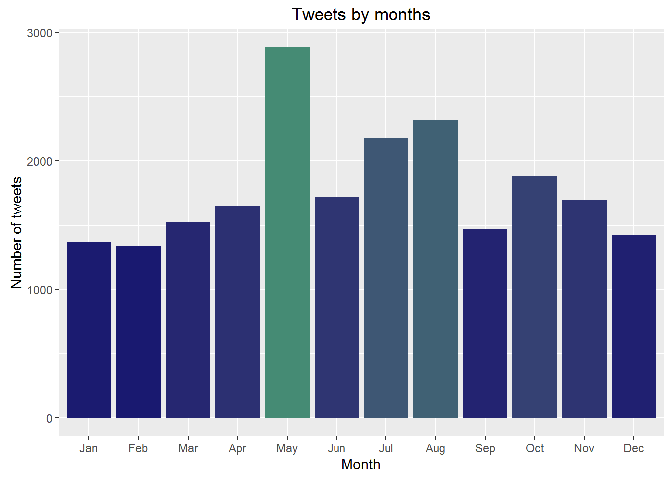 The month of May recorded the highest number of tweets.
ggplot(data = tweets, aes(x = wday(timestamp, label = TRUE))) +
geom_bar(aes(fill = ..count..)) +
ggtitle("Day of the week")+
theme(legend.position = "none") +
xlab("Day of the Week") + ylab("Number of tweets") +
scale_fill_gradient(low = "midnightblue", high = "aquamarine4")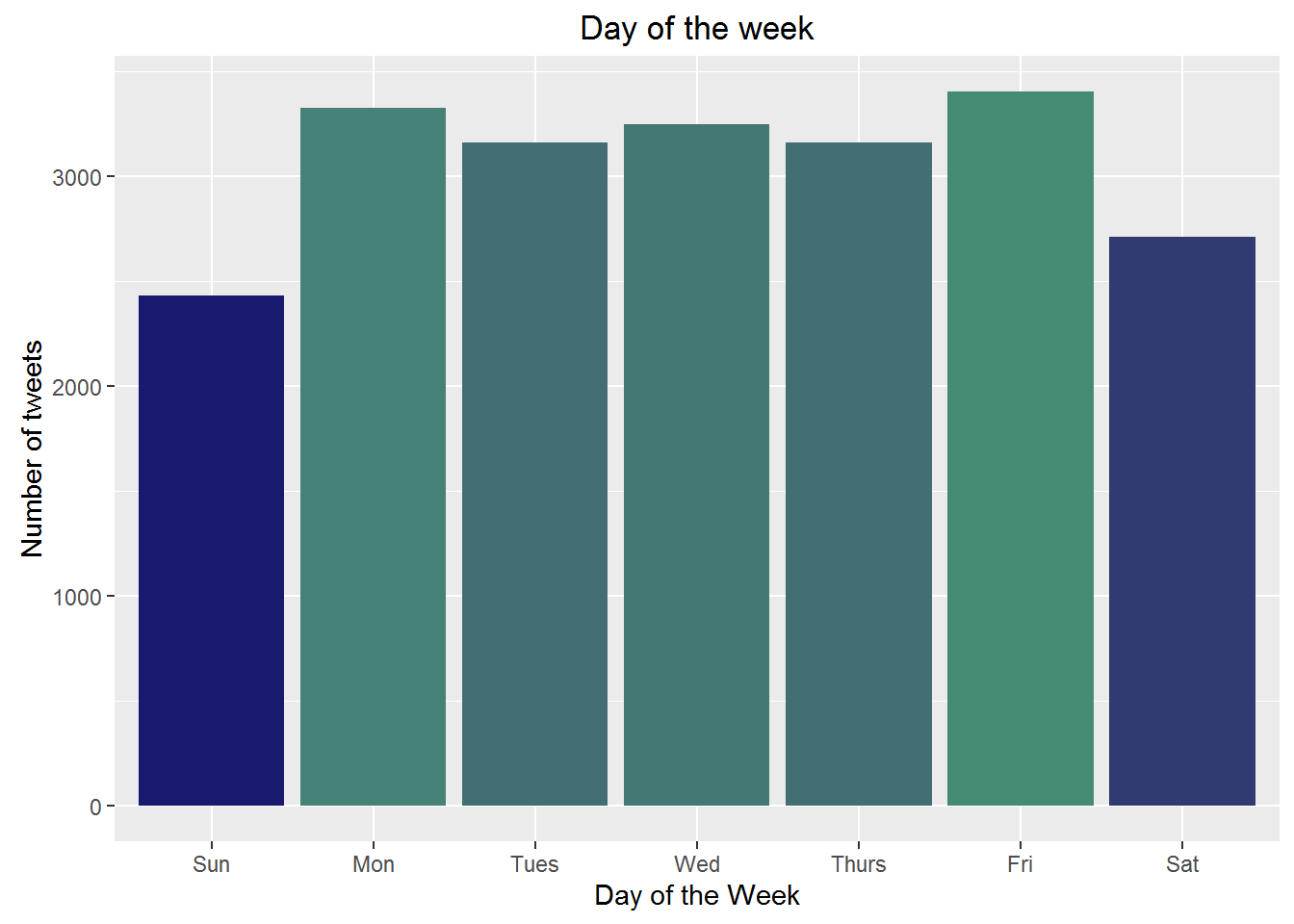 Monday and Friday turned out to be the most active days while Sunday ranked the lowest. Generally, tweeting frequency during weekdays was higher than during the weekend.
Further to this, it was apparent that mid morning and late evening were the best time for lordMwesh to tweet. Howerver, signficant tweeting appears to have taken place at 3am.
ggplot(data = tweets, aes(x = hour(timestamp))) +
  geom_bar(aes(fill = ..count..)) +
  theme(legend.position = "none") +
  ggtitle("Tweets by time of the day")+
  xlab("Time") + ylab("Number of tweets") +
  scale_fill_gradient(low = "midnightblue", high = "aquamarine4")
Lets get the number of retweets?
ggplot(data=tweets, aes(factor(!is.na(retweeted_status_id)))) +
geom_bar(aes(fill = factor(..count..)),  width = 0.3, stat="count") +
xlab("") + ylab("Number of tweets") +
ggtitle("Retweeted or Not") +
  theme(legend.position = "none") +
scale_x_discrete(labels=c("Not Retweeted", "Retweeted"))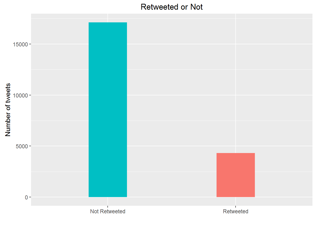
It happens that majority of lordMwesh’s tweets were “original” tweets.
How many tweets had hashtag compared to those without?
ggplot(tweets, aes(factor(grepl("#", tweets$text)))) +
        geom_bar(fill = "aquamarine4",width = 0.3) +
        theme(legend.position="none", axis.title.x = element_blank()) +
        ylab("Number of tweets") +
        ggtitle("Tweets with Hashtags") +
        scale_x_discrete(labels=c("No hashtags", "Tweets with hashtags"))
Which words does lordMwesh use frequently in his tweets?
nohandles <- str_replace_all(tweets$text, "@\\w+", "")
wordCorpus <- Corpus(VectorSource(nohandles))
wordCorpus <- tm_map(wordCorpus, removePunctuation)
wordCorpus <- tm_map(wordCorpus, content_transformer(tolower))
wordCorpus <- tm_map(wordCorpus, removeWords, stopwords("english"))
wordCorpus <- tm_map(wordCorpus, removeWords, c("amp", "2yo", "3yo", "4yo"))
wordCorpus <- tm_map(wordCorpus, stripWhitespace)

pal <- brewer.pal(9,"YlGnBu")
pal <- pal[-(1:4)]
set.seed(123)
wordcloud(words = wordCorpus, scale=c(5,0.1), max.words=100, random.order=FALSE,
          rot.per=0.35, use.r.layout=FALSE, colors=pal)
Will, can, Kenya and people are some of the frequently used words. The word “Internet” certainly had to make to this list considering lordmwesh’s zeal on matters Internet governance
Which twitter handles has lordmwesh interacted with more, either through reply or retweet?
friends <- str_extract_all(tweets$text, "@\\w+")
namesCorpus <- Corpus(VectorSource(friends))
set.seed(146)
wordcloud(words = namesCorpus, scale=c(3,0.5), max.words=50, random.order=FALSE,
          rot.per=0.10, use.r.layout=FALSE, colors=pal)
At least my name made to the list
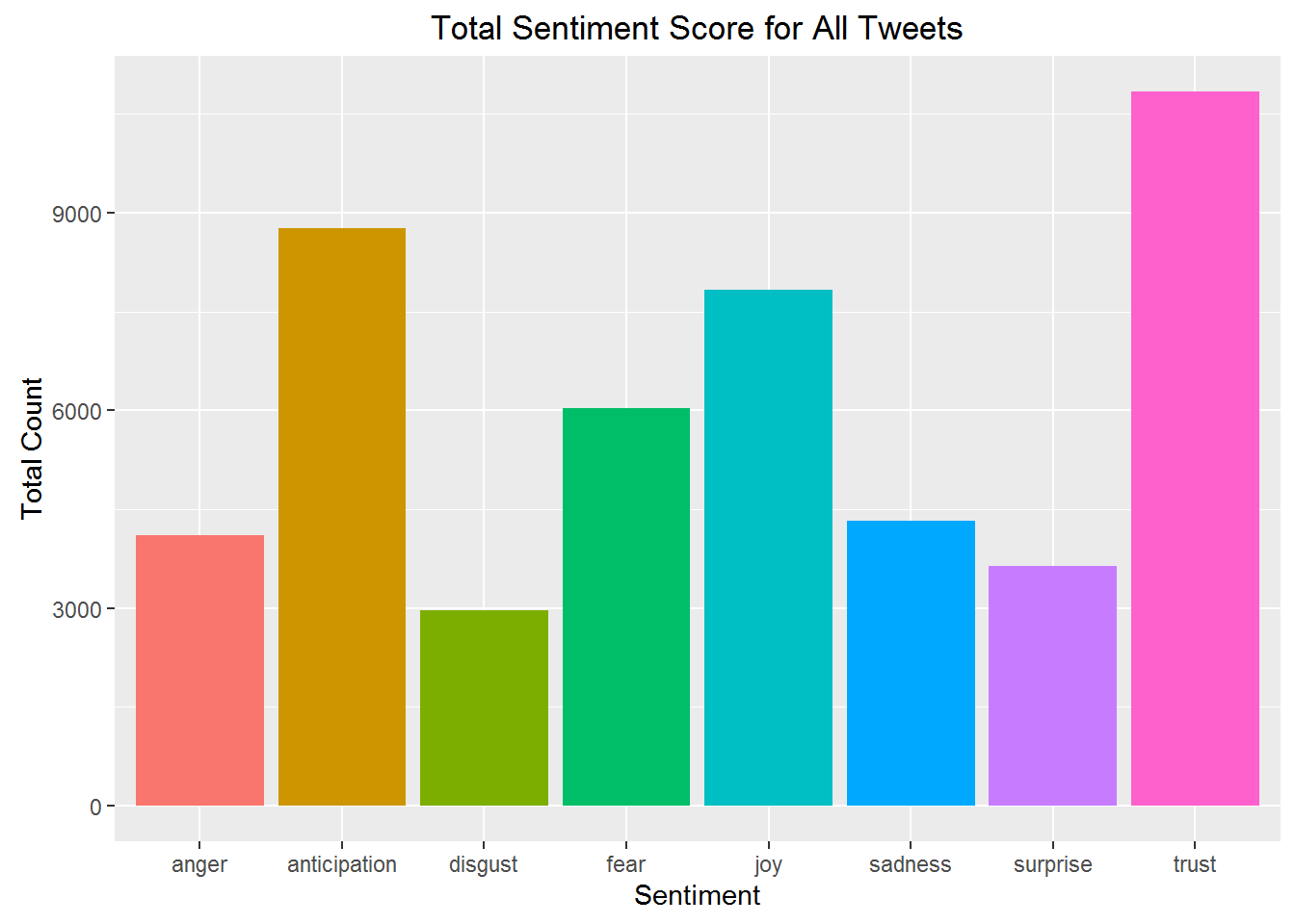
Sentiment Analysis
To evaluate and categorize the feelings expressed in text of the tweets, a sentiment analysis algorithm based on NRC Word-Emotion Association Lexicon was used.
lordmwesh_Sentiment <- get_nrc_sentiment(tweets$text)
tweets <- cbind(tweets, lordmwesh_Sentiment)
sentimentTotals <- data.frame(colSums(tweets[,c(11:18)]))
names(sentimentTotals) <- "count"
sentimentTotals <- cbind("sentiment" = rownames(sentimentTotals), sentimentTotals)
rownames(sentimentTotals) <- NULL

ggplot(data = sentimentTotals, aes(x = sentiment, y = count)) +
  geom_bar(aes(fill = sentiment), stat = "identity") +
  theme(legend.position = "none") +
  xlab("Sentiment") + ylab("Total Count") + ggtitle("Total Sentiment Score for All Tweets")